 Discusion Forums
 Courses
 AAnalyzer
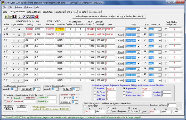
The most advanced methods for peak-fitting photoemission data are encompassed in AAnalyzer®. These are described in the five links below. With them, it is possible to obtain better fits and in a simpler way. Besides these methods, AAnalyzer® contains all the standard options of a photoemission fitting program (e.g., true Voigt functions, Doniach-Sunjic line shape, Shirley-Sherwood background, and the two and three-parameter Tougaard backgrounds, among others). All the parameters that it employs have a direct physical interpretation.
This is a very important tool in AAnalyzer® since it allows for a better modeling of the background. The active-background always provides better fits than the traditional method.
This is a variant of the Shirley-Sherwood background that does not require iterations and neither choosing two points. In this way, the fit and assessment of the peak areas become much less dependent on the operator.
This is a Tougaard-type background that models in a very simply way the change on the slope of the background between the two sides of the peaks. In combinations with the Shirley background, provides excellent fits for a wide range of spectrum shapes.
This provides an excellent option to the Doniach-Sunjic line shape. In contrast, the double-Lorentzian line-shape is integrable, allowing for quantitative analysis of the peak areas.
This is an excellent tool for discriminating overlapping peaks. It reduces enormously the uncertainty on the peak parameters values.
This section describes how to open files and plot them
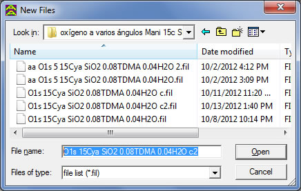
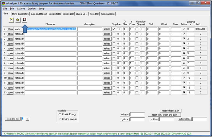
As soon as you open AAnalyzer, a pop up window will appear. This window will allow you to continue working on an existing project, it will open files with a .fil extension.

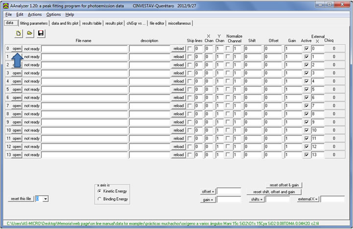
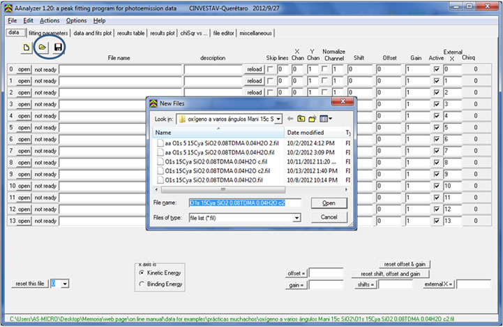
To start a new project, close the pop up window and choose the open button highlighted in the following image.
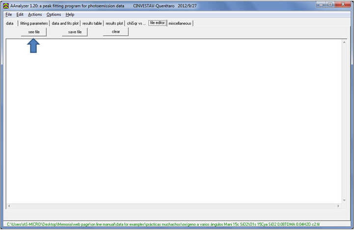
Now that the file has been selected, you must specify the data within the file that will be considered. Under the file editor tab, choose the “see file” option, and select the file that contains the experimental data.
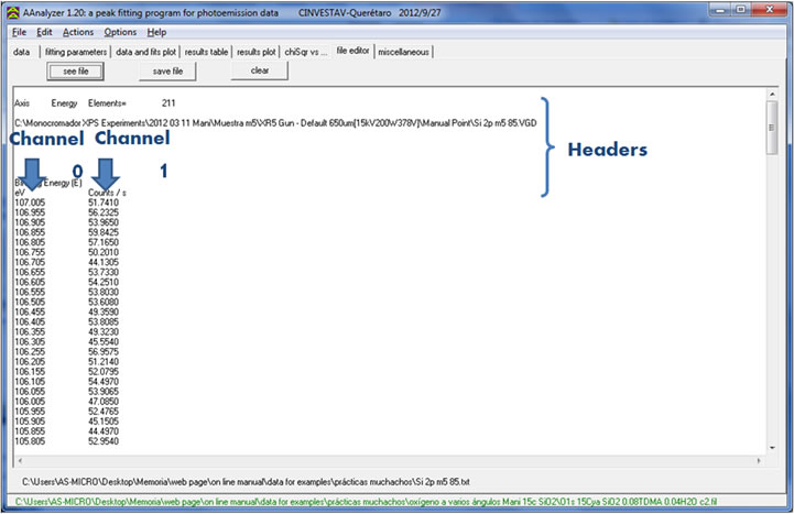
This option will allow you to open any text file. AAnalyzer will recognize columns (or channels) in the text file if they are separated by a coma, semi colon, space, or tab, as shown in the following image. Each channel represents a potential “x” or “y” axis.
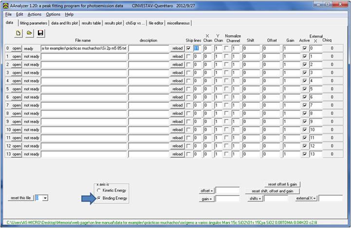
If your text file contains headers such as this one (as shown in the last image), you should check the skip lines box and indicate the number of lines covered by your headers. You must also indicate whether the channel corresponding to the “x” axis is binding or kinetic energy.
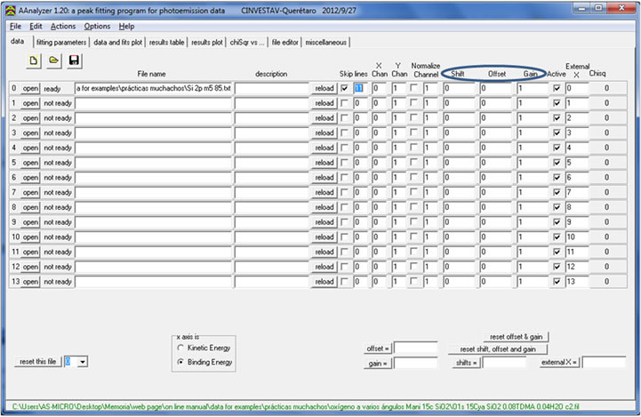
The “data” tab also allows the user to modify Shift, Offset, and Gain of the data. For more information about Shift, Offset, and Gain, please refer to the “Shift, Offset, and Gain options” instructional tab.
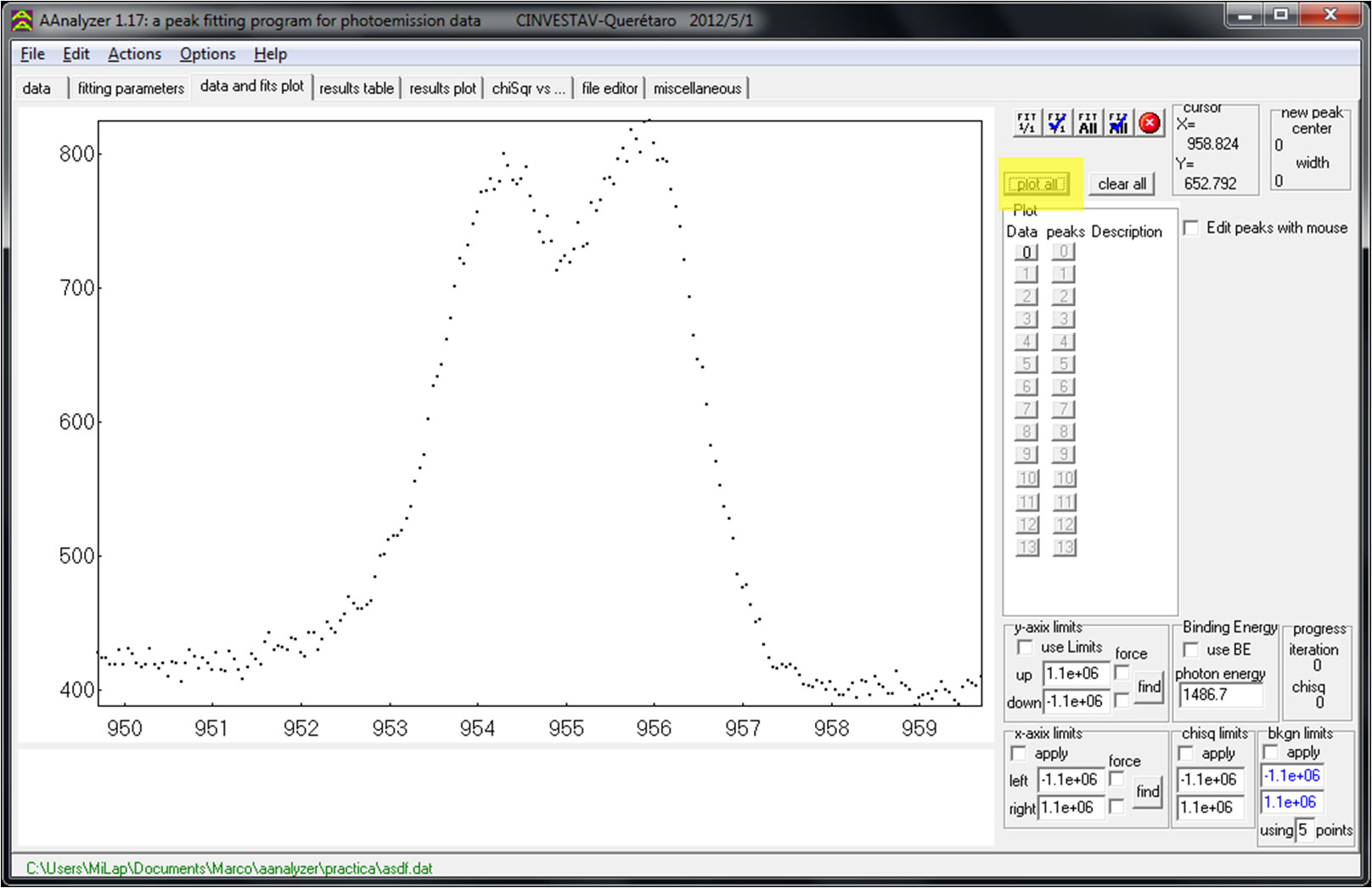
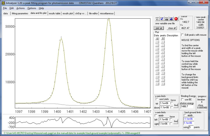
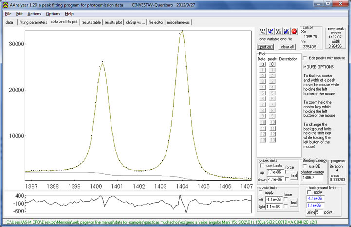
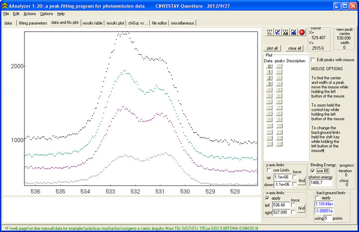
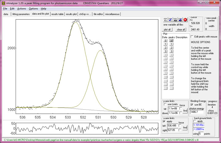
Finally, under the “data and fits plot” tab, click “plot all” to view your data on the graph. AAnalyzer will automatically plot the x axis as kinetic energy using the photon energy of Al K? (1486.7). If you wish that your x axis be shown as binding energy, check the “use BE” box near the lower left corner. If you used a different photon energy, make sure to input the proper value in the “photon energy” box.
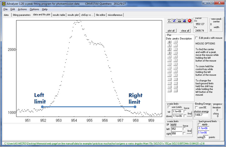
Should you want to zoom in to a certain area of your peak, you can either use the “x-axis limits” group box or use the mouse option. The first allows the user to reduce the “x axis” window in order to focus on a specific set of peaks. Input new “x axis” values in the “x axis limits” group box located near the lower left corner of the “data and fits plot” tab. Check the “apply” box and plot again.
If the “force” boxes are left unchecked, AAnalyzer will find “x axis” limits that better adjust to the peaks displayed for the given range. On the other hand, if the “force” boxes are checked, the “x axis” will be displayed with the exact limit values. Both options differ slightly. The “y axis” settings adjust automatically according to the data shown within the “x axis” limits.
With the mouse option, you may simply press-and-hold the “control” key and click-and-drag the mouse from the x-coordinates you wish to zoom in to. With this option you don’t need to click the “Plot All” button after selecting where to zoom in to.
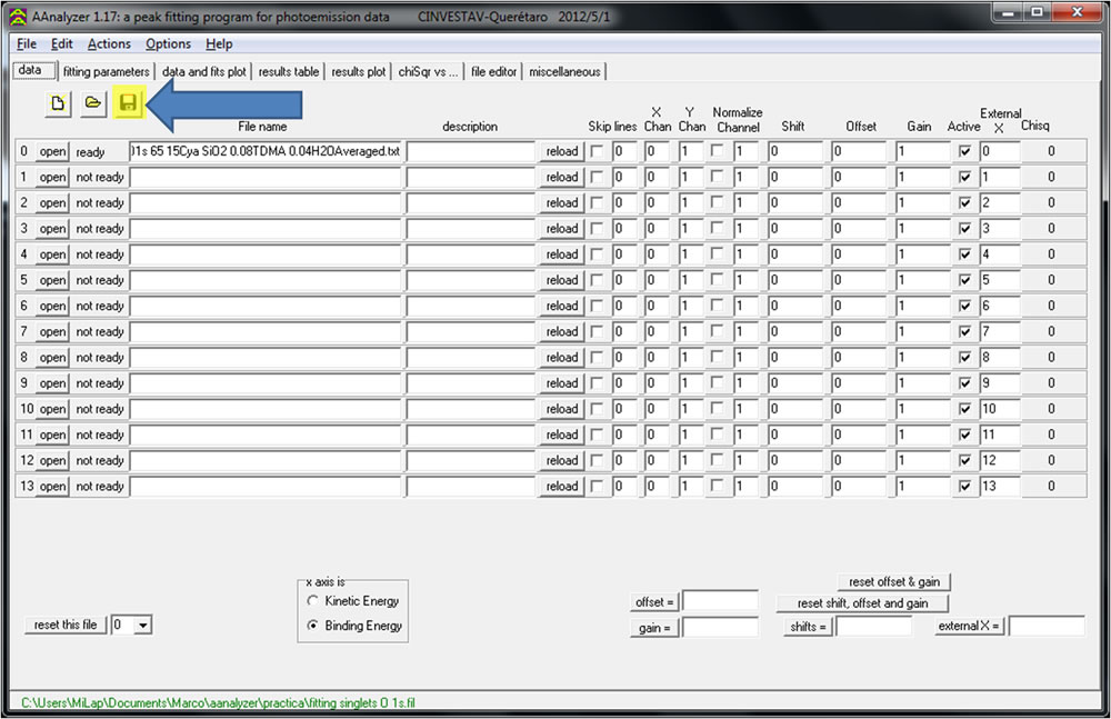
To save your progress, click the “save” button in the upper right corner of the “data” tab. This will save all information inputted in the “data” tab, as well as parameter information in the “fitting parameters” tab, if you have any. When you reopen AAnalyzer, you will be able to access any project you worked on by selecting it in the pop up window mentioned at the beginning of this section. The last project you saved will be the default file in the open box.
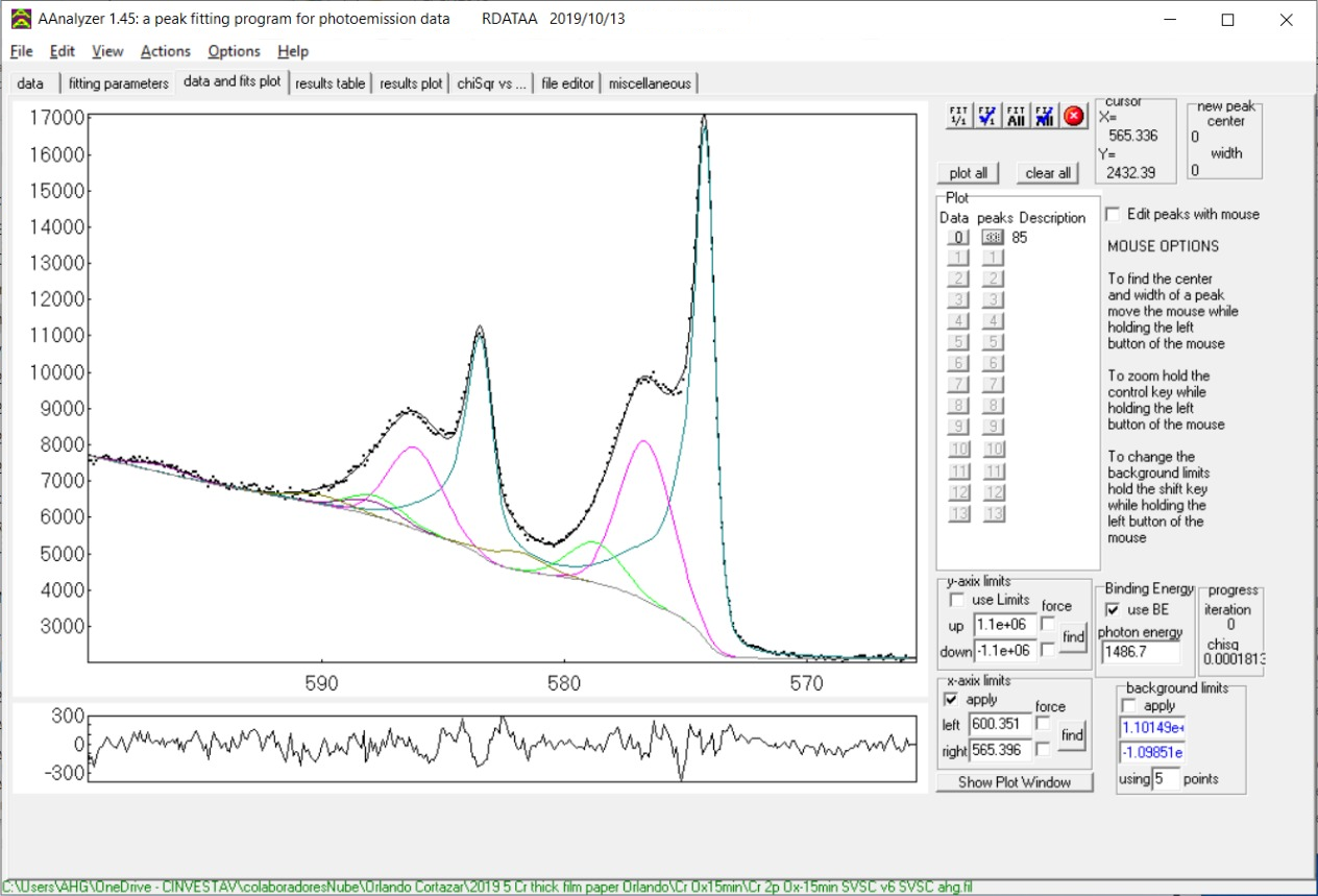
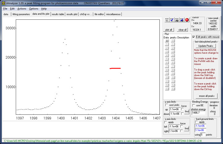
This section exemplifies a fitting process by employing an oxygen 1s spectrum containing two singlet peaks.
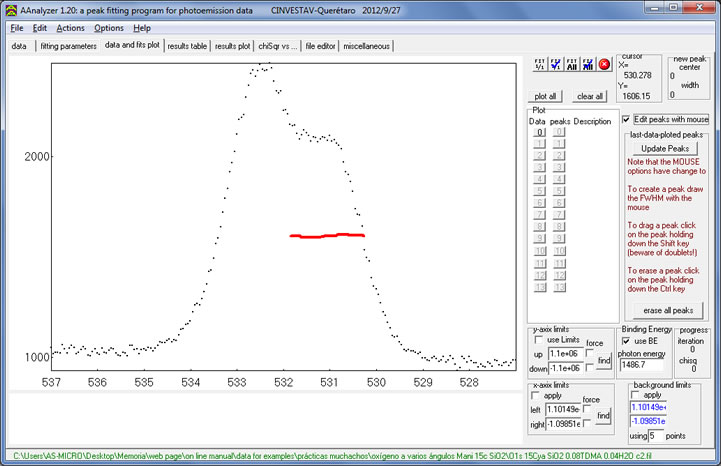
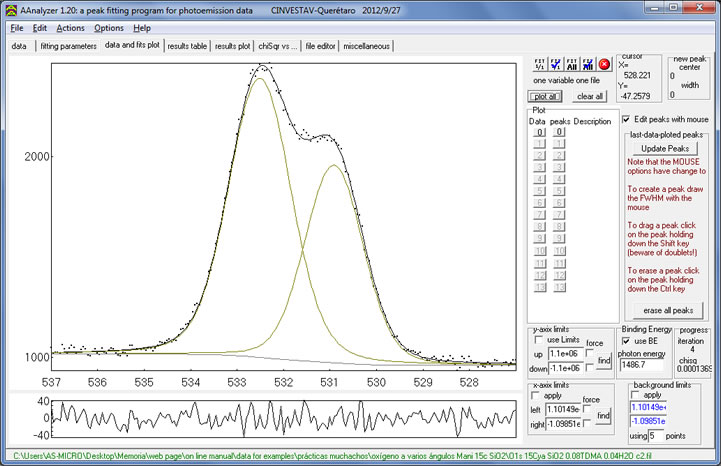
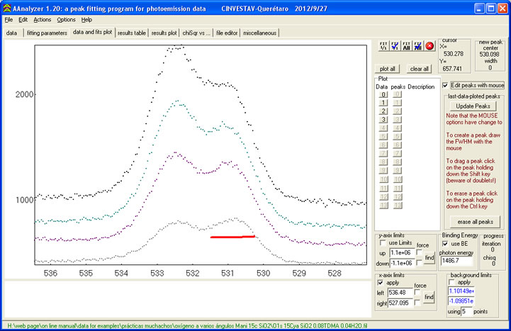
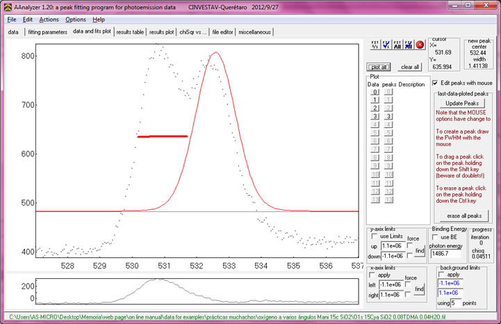
Once your data is plotted, you may create peaks by selecting the “edit peaks with mouse” box located on the right side of the window, and dragging the mouse across the width of the desired peak.
Repeat this process for as many peaks you might have.
To erase a bad peak or a miss-click, click the peak while pressing the “control” key. If you want to erase all the peaks drawn on the plot, press the “erase all peaks” near the lower left corner of the window. Once you have inputted your desired number of peaks, your window should look something similar to the following image.
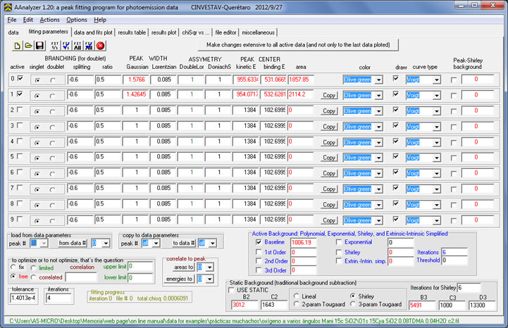
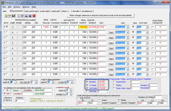
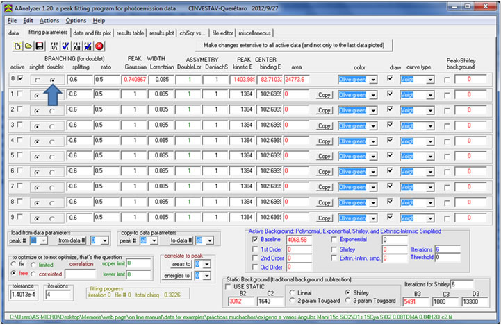
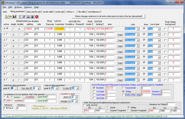
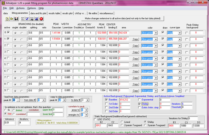
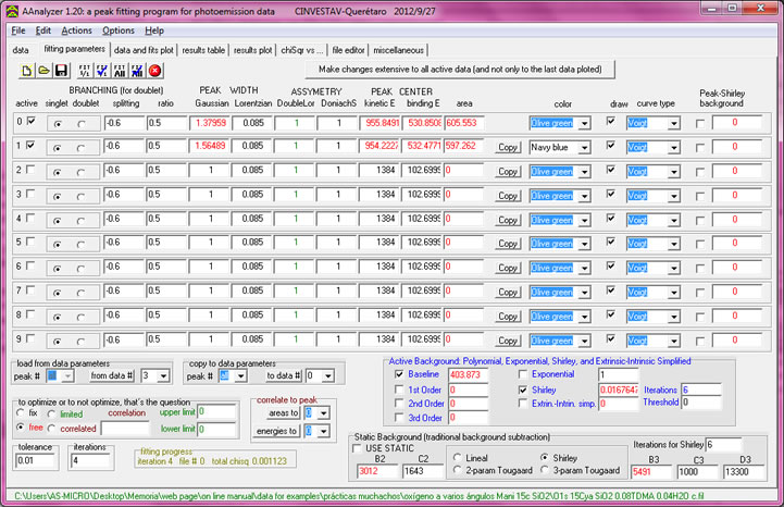
Back on the “fitting parameters” tab, AAnalyzer already created parameters for as many peaks that were created; you will be able to see these parameters at any time in the “fitting parameters” tab. Each row displays the parameters for an individual peak.
You may notice that some of the values in the “Fitting Parameters” tab are shown in red and others in black. The red font means that the values in these cells are “free”; these values will be modified by AAnalyzer when performing a fit in order to find an optimum value. The black values are “fixed”; these values will not change during a fit unless the user changes them. You may choose your values to be “fixed” or “free” by selecting the corresponding button near the lower left corner of the “Fitting Parameters” tab. The “limited” option does a similar function to the “free” function; however you must specify the limits in which AAnalyzer must optimize the value. On the other hand, the “correlated” option does a similar function to the “fix” function. This option will “fix” the value of the cell to the value of a different cell. To make reference to a different cell, take the first letter of the name of the column, and match it with its corresponding row number. For example, to make reference to the Gaussian cell of the first peak, input “g0”; -g- for Gaussian, and -0- for row #0. Specify the name of the cell you wish your value to be correlated to, in the space next to “correlated”. Examples of codes for all possible variables are found under the miscellaneous tab in the right side of the window.
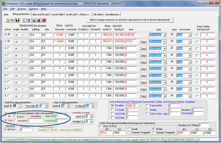
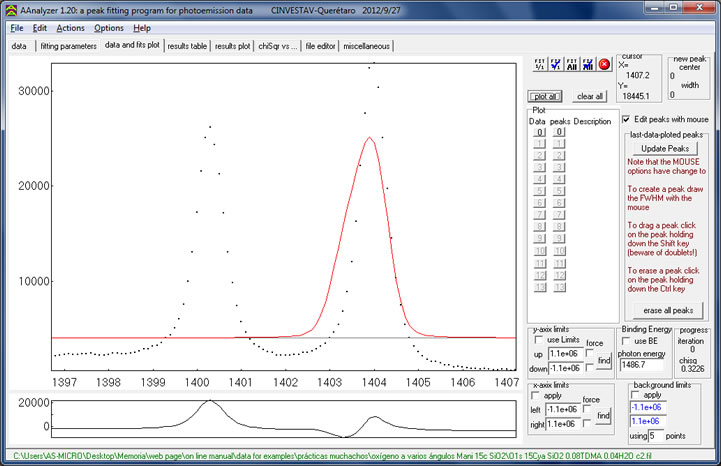
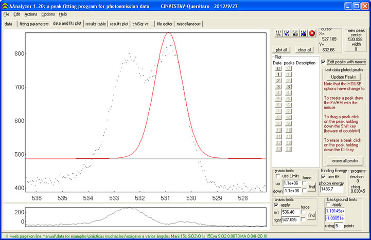
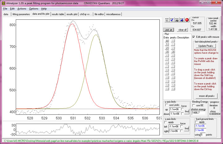
As you can see, the baseline was activated as soon as you inserted the first peak. AAnalyzer has as default the Active Baseline and Background option. Should you prefer to use the traditional (Static) background, select the "use static" checkbox beneath. For more information on active baselines and backgrounds please refer to the "Background Options" instructional tab. Make sure you check your desired background box. For this example, a Shirley background was selected.
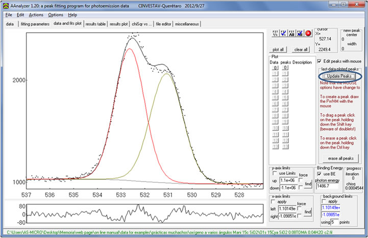
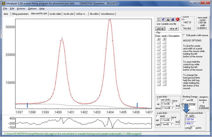
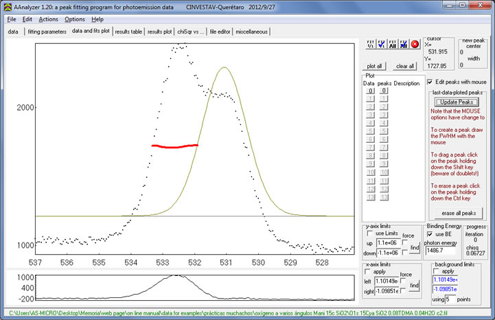
To visualize the modifications made for the baseline and background, click the “Update Peaks” button on the right side of the “data and fits plot” tab. (Remember that the “edit peaks with mouse” box should be checked for this button to be available.) Your peaks should look similar to the following image. Note that the peaks have not been fitted yet.
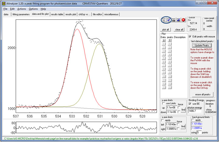
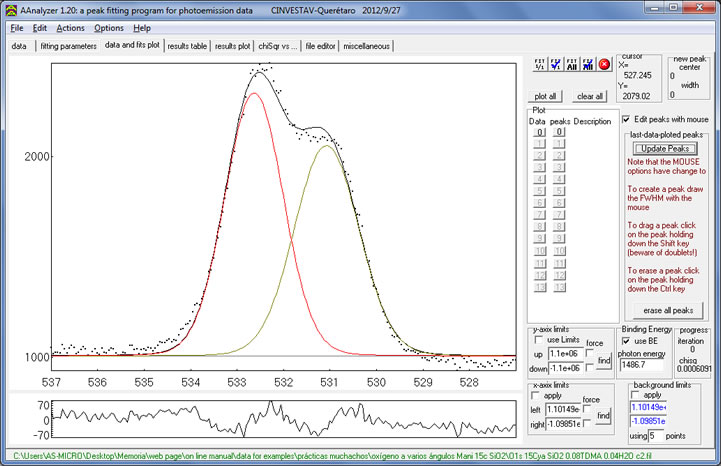
To begin the fitting process, click on any of the first two fitting buttons. Fit 1/1 – The first fitting option fits all “free” parameters (parameters in red font) simultaneously. This method provides a fast and efficient fit. Fit 1/1 ? – The second fitting option fits all parameters simultaneously as with the first button. Then, it fixes all free parameters except one and optimizes it individually. This process is repeated for as many “free” parameters you have (each time optimizing a different single parameter). This method provides a more precise optimized value for each parameter. For information about the function of the 3rd and 4th buttons please refer to the “simultaneous fitting” section.
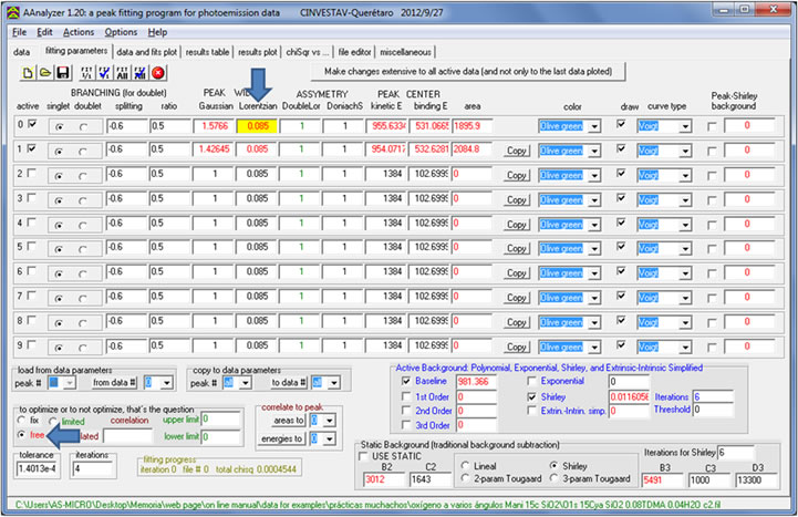
The fitting process is still incomplete at this point. AAnalyzer automatically fits all peaks using a “fixed” Lorenztian value of 0.085, which corresponds to the natural Lorentzian width of silicon 2p. However, the previous example displays two peaks from oxygen 1s, whose natural Lorentzian width is 0.25. Inputting known “fixed” values to your peak’s parameters will increase the accuracy of the fit. If you know the Lorentzian width of your core level, input the new Lorentzian value in the corresponding peak under the “fitting parameters” tab. Another option would be to set the value as “free”; this will allow AAnalyzer to find an optimum value. A. Herrera-Gomez, F.S. Aguirre-Tostado, M.A. Quevedo-Lopez, P.D. Kirsch, M.J. Kim, R.M. Wallace, J. Appl. Phys. 104 (2008) 103520.
Make sure to press one of the first two fitting buttons to visualize the changes made in the “fitting parameters” tab. The result is a much more precise fit, as shown in the following image.
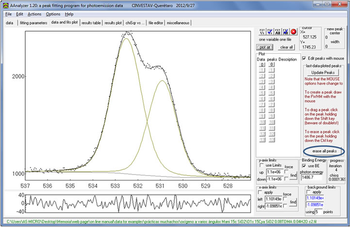
If you need to erase/deactivate any of your peaks, under the “data and fits plot” tab, click a peak while pressing the “ctrl” key to erase a specific peak, or press the “erase all peaks” button to erase all peaks displayed on the “data and fits plot” tab. Both of these functions are only available if the “Edit peaks with mouse” box is checked.
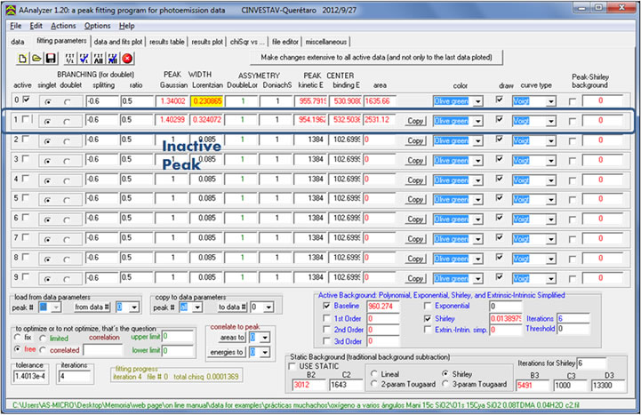
Ctrl-clicking a peak will only deactivate the peak in the “fitting parameters” tab. The next peak created will replace the deactivated peak. Under the “fitting parameters” tab, uncheck the corresponding “Active” box to deactivate a specific peak. This peak will stop displaying on the “data and fits plot” tab. To permanently erase all peaks, click the “clear all peaks” button near the top left corner of the “fitting parameters” tab. If you are working with more than one file, press the “Make changes extensive to all active data” button in the lower left corner of the window to apply the changes to the rest of the files.

To save your progress, click the “save” button in the upper right corner of the “data” tab. This will save all information inputted in the “data” tab, as well as parameter information in the “fitting parameters” tab. For more information about other saving options, please refer to the “Saving Options” instructional tab. When you reopen AAnalyzer, you will be able to access any project you worked on by selecting it in the pop up window mentioned at the beginning of this section. The last project you saved will be the default file in the open box.
This section explains how to use the different backgrounds available in the program.
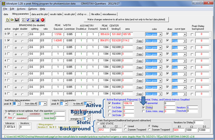
AAnalyzer counts with two different methods for reproducing a background. The Active Background method allows the user to employ several backgrounds simultaneously on a single fit. The Static Background (traditional) method allows the user to employ only one type of background at a time. Both methods are not compatible; selecting a method will automatically disable the other. All background options are located under the “fitting parameters” tab and can be selected by simply checking the box next to your desired background.
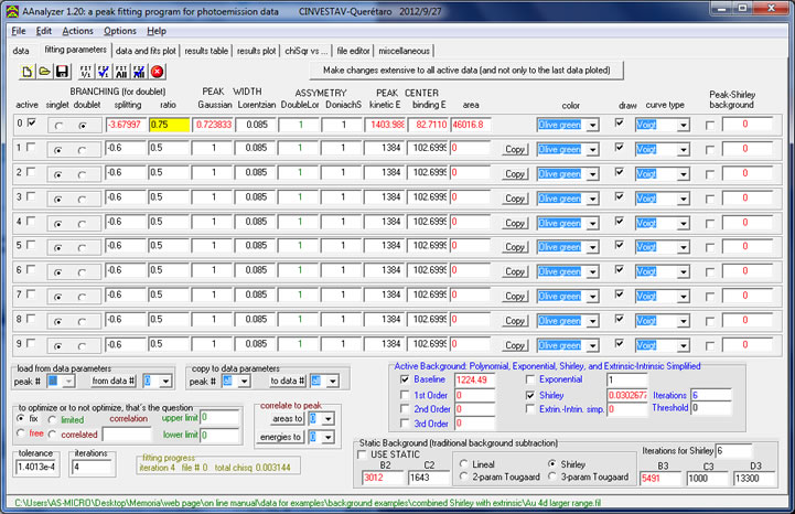
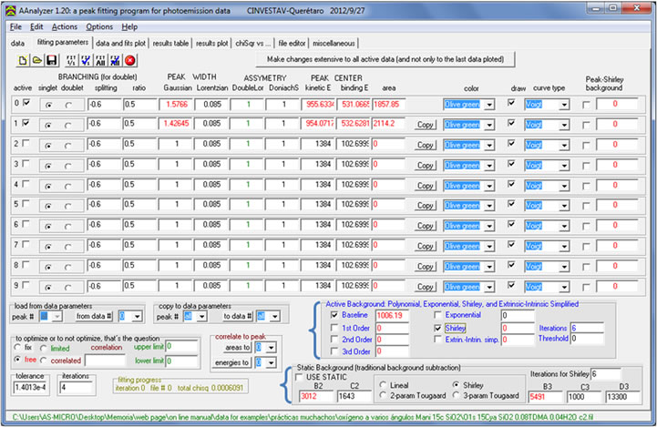
One of the unique features of AAnalyzer is the Active Background, which allows the user to fit with one or several different backgrounds simultaneously. In order to activate the Active Background, check any of the background boxes under the “Active Background” group box, as shown in the following image. Beware that selecting too many backgrounds from the “active Background” group box may not be beneficial, as it involves too many variables and it decreases the accuracy of the fit.
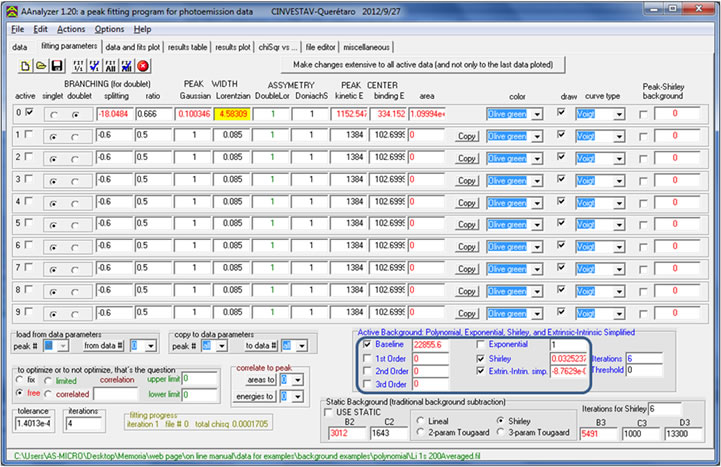
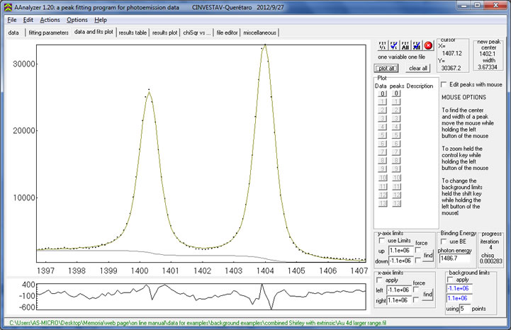
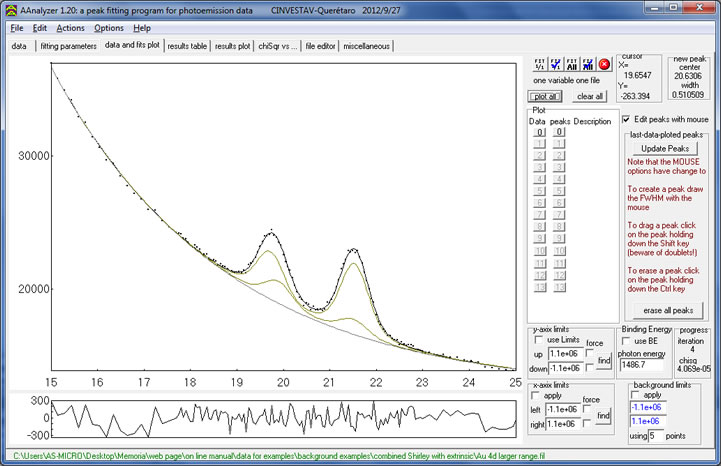
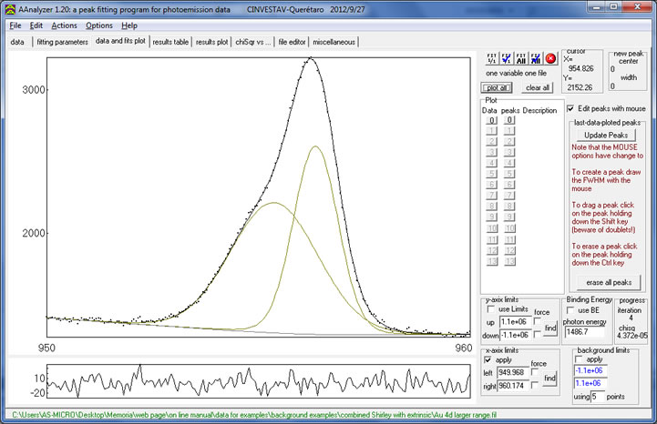
The following example is a Au 4d spectra fitted with an Active Background combination of Shirley and Extrinsic Simplified backgrounds (aside from the baseline). The types of backgrounds available for Active Background combinations are explained later on in this section. Please note that an Active Background allows employing one or several backgrounds at a time.
The user has several background options to choose from in the Active Backgrounds group box. These options are described below.
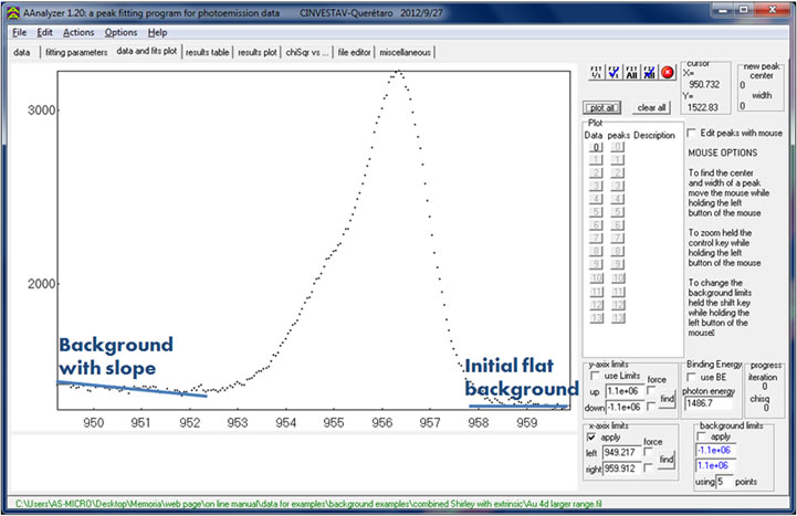
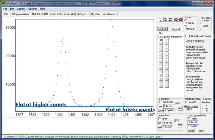
How to identify: The Extrinsic Simplified Background is also a unique feature of AAnalyzer. It is similar to the Shirley background; however, instead of producing a flat elevated background to the left of the peak, the background tilts upwards or downwards with a constant slope, as shown in the following image.
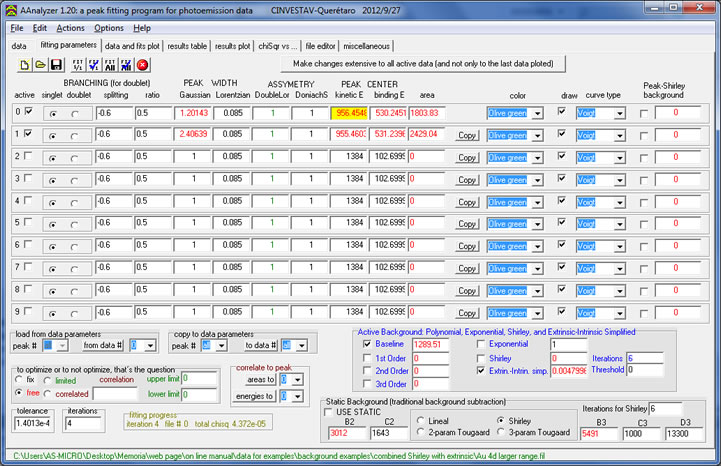
This example of an O1s displays an initial flat background to the right and a negatively sloped background to the left of the peak. These characteristics are well reproduced with an Extrinsic Simplified background as shown in the following images.
Graphic example
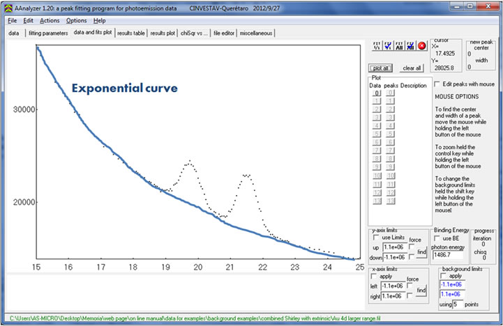
How to identify: An exponential Background is more commonly found at low electron kinetic energies. This background grows exponentially to the left.
The background for this example (Sr 3d acquired with is 130 eV photon energy) is well reproduced with an Exponential Background, as shown in the following images.
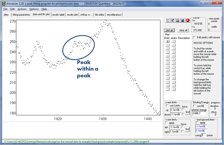
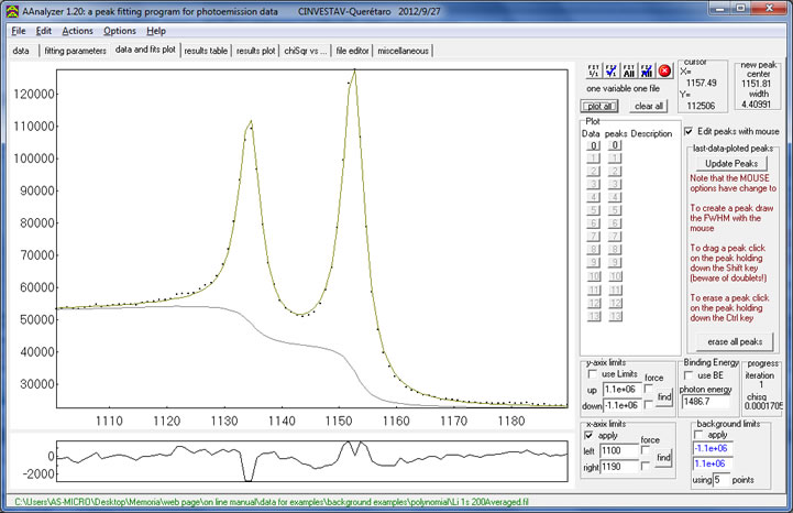
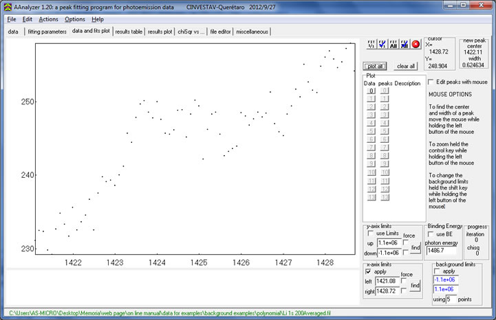
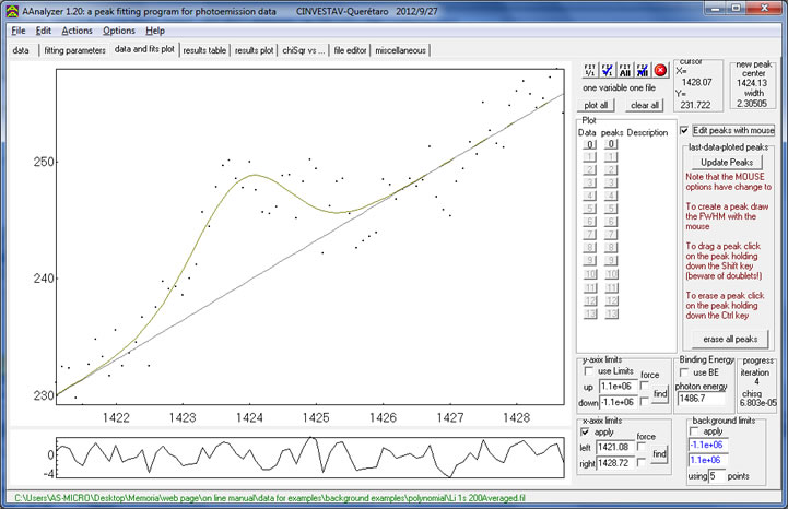
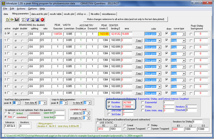
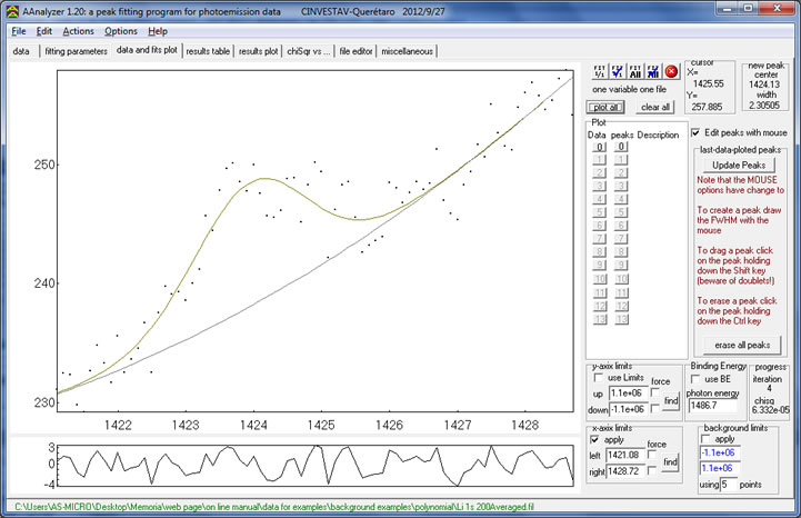
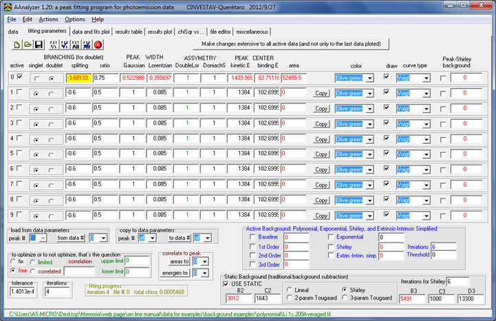
How to identify: Linear and Polynomial Backgrounds are used when none of the previously described type of backgrounds is able to reproduce the data. This is mostly the case for when the peak rides on top of the background of another more dominant peak. The following is an example of a small Li 1s peak on top of the background from a silicon oxide sample.
Graphic example
Graphic example
Graphic example
Both the Linear and the Polynomial backrgrounds are able to reproduce this background example of a Li 1s spectrum.
To activate a Static Background, check the “use static” box and choose the type of background you wish to use. Checking the “use static” box will disable the “Active Background” group box. The following example is a Au 4f spectrum fitted with a Shirley Static background.
Graphic example
Fitting a doublet peak is a very similar process to that of a singlet. Once the data of your doublet peak is plotted, you may draw the peak by selecting the “edit peaks with mouse” box located on the right side of the window, and dragging the mouse across the width of the desired peak (Note that you only have to input one peak when Fitting doublets). Your window should look like the following images.
If you are having trouble drawing a peak, please refer to the “open files” and/or “Fitting singlet peaks” instructions.
Once you have inputted your peak, AAnalyzer will create parameters for your new peak in the “fitting parameters” tab. Each row represents the parameters for a peak. Under this tab, make sure to specify that your peak is a doublet. Also make sure to add a background (refer to “Fitting Singlet Peaks” instructions for more information about baselines and backgrounds).
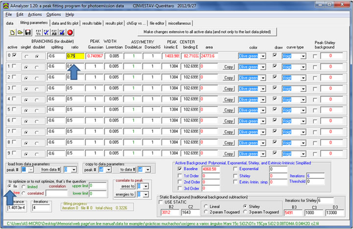
The final steps before beginning the fitting process are to specify the splitting and the ratio of your peak. If you already know the branching ratio of the doublet (0.5 for p-type, 0.666 for d-type, and 0.75 for f-type), indicate it on the “ratio” cell located near the upper left corner of the window. Make sure that you set the ratio as “fix”. This will ensure an optimum fit of your peak without modifying the “ratio” value.
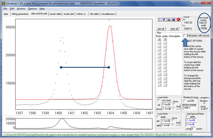
Then, input the value of the splitting in the splitting box located under the “Fitting Parameters” tab. If you need assistance to determine an approximate value of the splitting, uncheck the “edit peaks with mouse” box under the “data and fits plot” tab, and click-and-drag your mouse from the crest of one branch to the other. This will give you an approximate difference between the two centers of energy. This difference will be shown as a “width” value in the upper right corner of the “data and fits plot” tab.
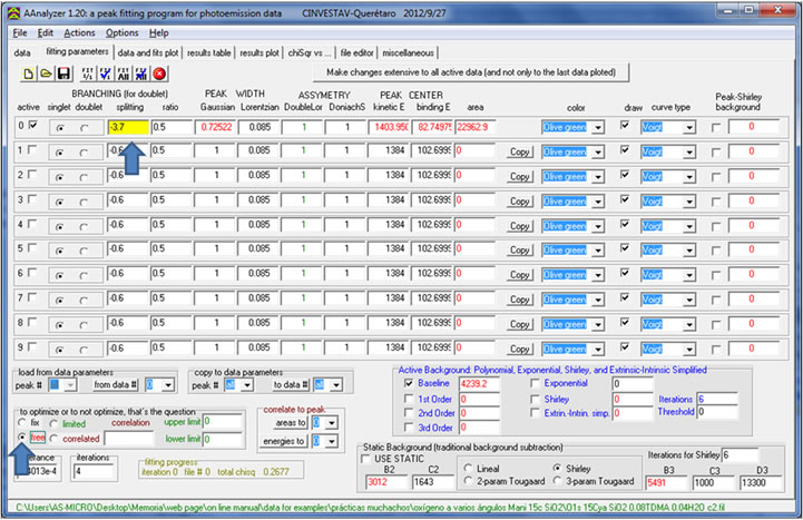
Make sure that you select the “splitting” as a “free” parameter; this will allow AAnalyzer to find an optimum value of the splitting.
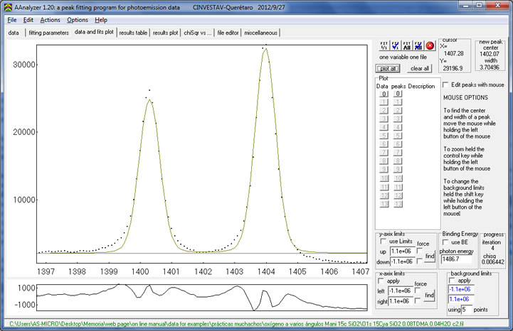
To begin the fitting process, press any of the first two fitting buttons located on the upper right corner of the window under the “data and fits plot” tab. Both branches are fitted with the same lorentzian and gaussian values. Fit 1/1 – The first fitting option fits all “free” parameters (parameters in red font) simultaneously. This method provides a fast and efficient fit. Fit 1/1 ? – The second fitting option fits all parameters simultaneously as with the first button. Then, it fixes all free parameters except one and optimizes it individually. This process is repeated for as many “free” parameters you have (each time optimizing a different single parameter). This method provides a more precise optimized value for each parameter. For information about the function of the 3rd and 4th buttons please refer to the “simultaneous fitting” section.
The fitting process is still incomplete at this point. AAnalyzer automatically fits all peaks using a “fixed” Lorenztian value of 0.085 eV, which corresponds to the natural Lorentzian width of Si 2p. However, the previous example displays a doublet of Au 4f, whose natural Lorentzian width is approximately 0.42 eV. Inputting known “fixed” values to your peak’s parameters will increase the accuracy of the fit. If you know the Lorentzian width of your core level, input the new Lorentzian value in the corresponding peak under the “fitting parameters” tab. Another option would be to set the value as “free”; this will allow AAnalyzer to find an optimum value.
Make sure to press one of the first two fitting buttons to perform a fit and visualize the changes made in the “fitting parameters” tab. The result is a more precise fit.
To save your progress, click the “save” button in the upper right corner of the “data” tab. This will save all information inputted in the “data” tab, as well as parameter information in the “fitting parameters” tab. For more information about other saving options, please refer to the “Saving Options” instructional tab. When you reopen AAnalyzer, you will be able to access any project you worked on by selecting it in the pop up window mentioned at the beginning of this section. The last project you saved will be the default file in the open box.
All saving options may be accessed under the “file” drop menu.
This option saves an AAnalyzer project. It records every modification/adjustment made in the “data” tab, as well as all peaks and parameters on the “fitting parameters” tab. These files (.fil) can be accessed with the initial pop-up window, or by clicking the “open project” button on the “data” tab.
This option saves the parameters of all active peaks in the “fitting parameters” tab. These files (.par) can be uploaded into AAnalyzer using the “Open Parameters” button near the upper-left corner of the “fitting parameters” tab, or they can also be viewed using any text editing software.
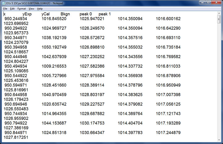
This option saves the following project information into channels: “x axis”, experimental data, final fit, background, peak 0, peak 1, peak 2, and so on, and can be viewed with any text editing software. These files (.fit) save information of only one file on the “data” tab.
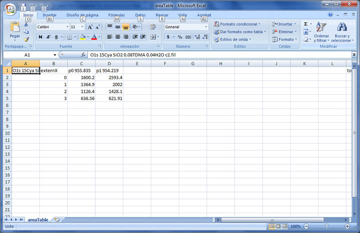
This option saves the current table displayed in the “results table” tab. To save a table with a different parameter, select the new parameter on the “results for” drop box and save. These files (.tbl) can be viewed with any text editing or spread sheet software (such as Microsoft Excel). For more information about the “results table” please refer to the “Using the results table and results plot” instructional tab.
All saving options may be accessed under the “file” drop menu.
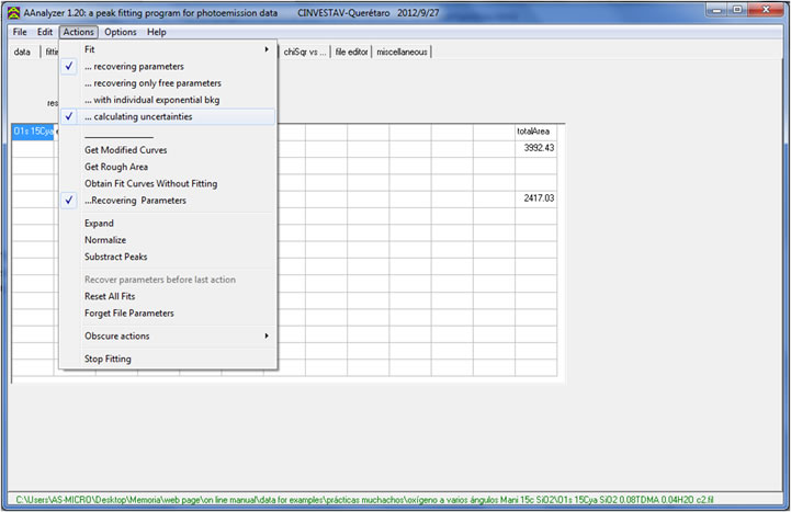
This function is available in the “Results table” tab; however, it needs to be activated prior to making the fit. Under the “Actions” drop menu, press “…calculating uncertainties” to activate it.
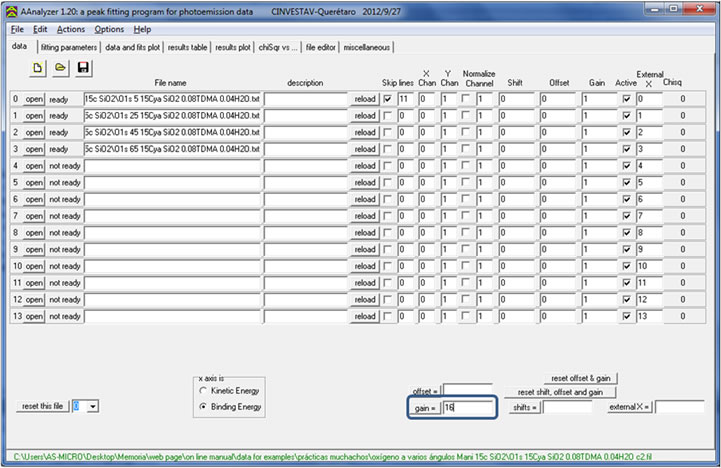
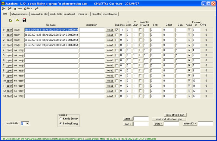
By activating the uncertainties function, AAnalyzer automatically assumes Poisson Statistics. Make sure to set an appropriate “gain” in order to indicate total count values instead of normalized count values. This can be done in the “data” tab. After inputting a “gain” value, press the “gain=” button, to apply it to all the files in the “data” tab. The gain value should be the product of the dwelling time and the number of scans.
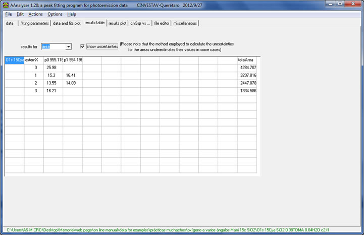
Once you have set a “gain” value, fit the data once more; this time, AAnalyzer will calculate uncertainties while performing the fit. For more information about how to perform a fit, please refer to the “Fitting singlet peaks” or “Fitting multiple files” instructional tabs. This example shows the uncertainties of the Gaussian width of “peak 0” and “peak 1”
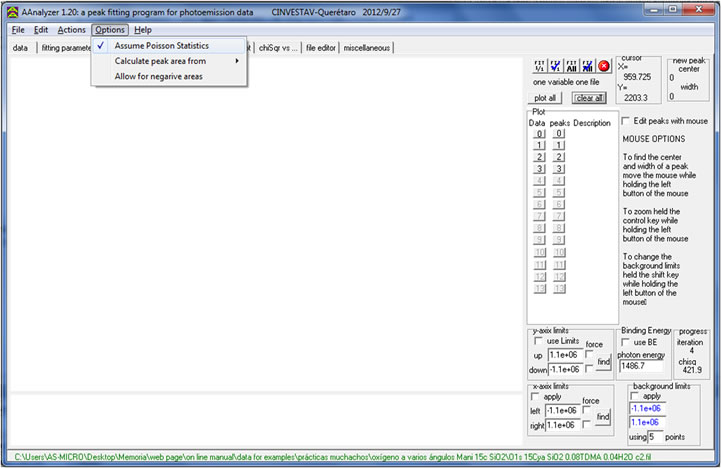
To remove Poisson Statistics, uncheck the “Assume Poisson Statistics” option by selecting it under the “Options” drop menu.
AAnalyzer counts with unique algorithms for fitting multiple files. These apply when fitting several spectra of the same type, such as Ti 2p spectra obtained from samples with different processing parameters. This section will explain different ways to fit multiple files using as an example O 1s spectra obtained at various angles.
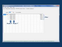
AAnalyzer allows the user to plot several files on the “data and fits plot” tab. This can be done by uploading more files onto AAnalyzer in the “data” tab. Each row on the “data” tab represents an individual file. Press the “open” button and select the file that you want to upload (you may add up to 14 files). For a better functionality, the spectral range of all uploaded files should be similar. Make sure to indicate whether the channel corresponding to the “x” axis is binding or kinetic energy. For more information about how to upload files, please refer to the “open and plot files” instructional tab.
Once you have uploaded your desired number of files, press the “plot all” button located near the upper right corner in the “data and fits plot”; you should be able to see all data from all your files on the plot. As you can see, the "use BE" box is checked. This changes the horizontal scale from kinetic to binding energy employing the photon energy indicated in the box below the "Use BE" checkbox.
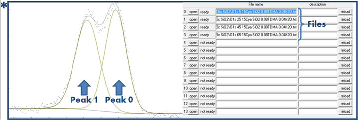
Once you have the data plotted, you may begin drawing the peaks (this process is also described in the “fitting with singlet peaks” instructional tab). Check the “edit peaks with mouse” box in the right side of the window, and click-and-drag across the width of the peak. Repeat this process for as many peaks you might have. Note that you only need to draw the peaks for only one file; AAnalyzer will automatically use the parameters of these peaks and apply them to the rest of the files.
Please note how AAnalyzer has automatically placed a baseline for your peak. The parameters for the baseline can be seen in the "Fitting Parameters" Tab in AAnalyzer.
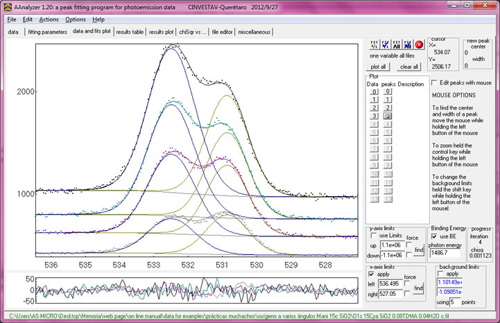
Once you begin drawing peaks, the plot will only show data from the last file plotted. This will avoid a crowded-looking plot. However, you can still see all the data from all the files by clicking the corresponding “data button(s)”, as shown in the following image.
To return to the original setting, press the “clear all” button, and then press the last data button to plot the data (in this case, it was data 3), as well as its corresponding peak button. You can continue drawing the peaks at any time.
Note that the color of the peaks changes to facilitate visual distinction. Once you are done drawing your peaks, your window should look similar to the following image.
Under the “fitting parameters” tab, add the background you need. For more information about how to add baselines and backgrounds, please refer to the “Fitting singlet peaks” or “Background options” instructional tabs. As you can see, AAnalyzer uses as default the Active Baseline and Background option. Should you wish to use the traditional (Static) option, simply click the "USE STATIC" checkbox beneath.

To begin the fitting process, press any of the fitting buttons located on the upper right corner of the window under the “data and fits plot” tab. Fit 1/1 – The first fitting option fits all free parameters for all files, one file by one, in a sequential manner. Each file will have its own set of fitting parameter values. Fit 1/1 ? – The second fitting option also fits all free parameters for all files, one file by one, in a sequential manner; however, it provides more precise parameter values. Likewise, each file will have its own set of fitting parameter values. Fit all – The third fitting option fits all “free” parameters (parameters in red font) of all files simultaneously. The center and width of the peaks are fitted to the same values for all the data; however, it allows for different peak areas. This method provides a fast and efficient simultaneous fit. Fit all ? – The fourth fitting option fits all parameters simultaneously of all files, as with the third option; however, it provides a more precise optimized value for each parameter.
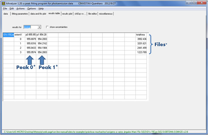
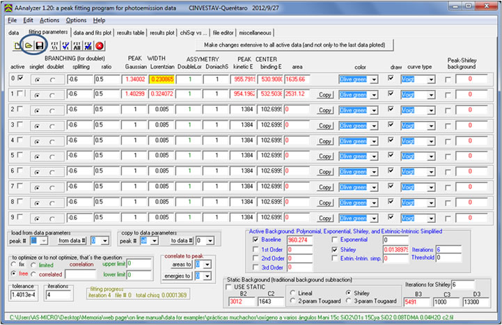
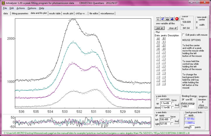
The main difference between the first pair (sequential fitting) and the second pair of fitting options is that the second pair fits the data of all files with a unique process called “simultaneous fitting”. Simultaneous fitting means that for each peak created, AAnalyzer will recreate the peak in each file with the exact same center and width. This can be further explained with the “results table” tab. For more information about how to use the results table, please refer to the “Using the Results Plot and Results Table” instructional tab. The results table allows the user to compare values of a single parameter from the same peak located in different files. Each row represents a file while each column represents a peak. When fitting sequentially, AAnalyzer optimizes energy and width values (among other parameters) individually. This means that there will be a different optimized energy value for the same peak found among different files, as shown in the following image

This example of a sequential fit provides optimized energy values with slight differences for each peak among the different files. “Resolving overlapping peaks in ARXPS data: The effect of noise and fitting method.” J. Muñoz-Flores, A. Herrera-Gomez, J. Electron Spectrosc. Relat. Phenom. 184 (2012) 533.
When fitting simultaneously, AAnalyzer optimizes energy and width values conjunctly. This means that the energy and width values for a peak among different files will be exactly the same, as shown in the following image.
Simultaneous fitting increases the accuracy of the peaks’ parameters. Having a single value of energy for the same peak in different files is also a more accurate interpretation of the spectrum taken at different angles. On the other hand, if one were to fit all peaks sequentially, the energy centers would still be relatively close, but the fitting process is prone to more uncertainties due to the differences in energies of the same peak.
Back on the data tab, press either the 3rd or 4th fitting button to get a simultaneous fit, or the 1st or 2nd fitting button to get a sequential fit. The following example was fitted simultaneously.
After fitting, AAnalyzer will only show the data and peaks from the last file in the list. Press “plot all” to see the data from all the files.
To see peaks from an individual file on the plot, press the “peak” button corresponding to the file you desire.

To load the peak’s parameters from an individual file into the “fitting parameters” tab, select the file from the drop box next to the “from data #”, located in the “fitting parameters” tab. Please note that “data 0” refers to your first file in the “data” tab, and “data 1” refers to your second file, and so on. Once you have selected your desired file, press the “from data #” button near the top edge of the window to load the peak’s parameters. The parameters can also be viewed and displayed in the “results table” and “results plot” tabs. For more information, please refer to the “Using the “results table” and “results plot”” instructional tab.
To save your progress, click the “save” button in the upper right corner of the “data” tab. This will save all information inputted in the “data” tab, as well as parameter information in the “fitting parameters” tab. For more information about other saving options, please refer to the “Saving Options” instructional tab. When you reopen AAnalyzer, you will be able to access any project you worked on by selecting it in the pop up window mentioned at the beginning of this section. The last project you saved will be the default file in the open box.